Why was the severe storms outbreak on 14 November 2011 lacking in tornadoes whereas the outbreak two days later had multiple tornadoes? Despite the SPC outlook highlighting a 10% tornado probability contour with the potential for significant tornadoes (black hatching in the bottom left of Figure 1), almost no tornadoes occurred. Two or three tornadoes were later confirmed in southwest New York but those fell outside of the region of significant tornado threat stretching from southern Illinois to far western Pennsylvania. Two days later, multiple tornadoes were reported from Alabama to North Carolina even though the forecasted tornado probabilities were somewhat lower. I document the comparisons between these two events with a specific interest in finding differences that may lead to different outcomes than what was forecast. As a note, I consider SPC convective storms outlooks to be the state of the art of our science of forecasting these events and so it serves as a useful benchmark. So when events occur where an outcome is different than what's expected from these forecasts then something really useful can be learned.
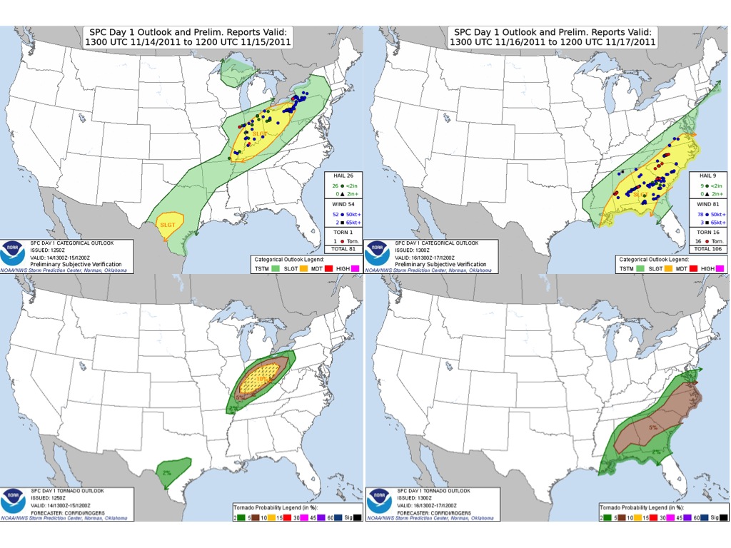 |
| Figure 1. Local Storm Reports (LSRs) overlaid for the verification time of the categorical SPC day 1 outlook made 13 UTC for 14 November 2011 (top left) and 16 November 2011 (top right). The bottom two panels show the accompanying tornado probability forecasts. |
 |
| Figure 2. A four panel display of the morning 500 mb analysis and observations for 14 November (upper left) and 16 November (upper right). The 925 mb level is displayed in the bottom two panels. Source: SPC. |
The clash of the air masses hypothesis now indicates that the 14th should be more tornadic. Perhaps I'm being a bit sarcastic by bringing up this term but I hear it promoted all too frequently. As we've already stated, the 14th was not the bigger tornado day and we already have seen that the most tornadic convection on the 16th didn't form on anything really resembling a front.
 |
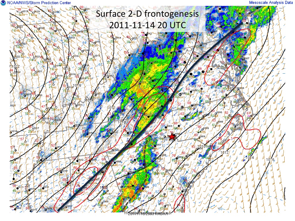
| Figure 3. Surface 2-D frontogenesis, surface plot and mosaic radar reflectivity for 20 UTC 14 November 2011. The thin black contours represent sealevel pressure while the thick blue line marks the cold front. Source: SPC |
 |
| Figure 4. Like Figure 3 except for 16 November. |
 |
| Figure 5. 100 mb mixed layer CAPE (MLCAPE) and MLCIN for 14 November 2011 - 20 UTC. Areas devoid of blue shading while exhibiting positive MLCAPE suggests an atmosphere with no or little CIN. The red star indicates a RUC analysis sounding shown below. |
 |
| Figure 6. Similar to figure 5 except for 16 November |
The cursory analysis of CAPE and CIN appeared to be sufficient for convective storms to form, and the shear certainly seemed sufficient to allow supercells to form if updrafts were allowed to properly interact with the shear. At least 40 kts of vertical wind shear would boost the prospects for supercells quite to the point that forecasters would expect them to form. Both 14 and 16 November had sufficient deep layer shear as implied by the bulk wind difference plots in the lowest half of the convectively active layers as Figures 7 and 8 show. In fact the 14th had nearly 80kts of bulk wind difference in the 0 - 6 km layer (a proxy for vertical wind shear).
 |
| Figure 7. Effective bulk wind difference for 14 November 2011 - 20 UTC. Source: SPC. |
 |
| Figure 8. Similar to figure 7 except for 16 November - 22 UTC. |
The only two environmental parameters to check would be boundary layer RH with mixed layer LCL as a proxy, and the vertical bulk wind difference in the 0-1 km layer. Instead of going through both of those plots, let me say that the MLLCL was near the optimal values of 700 m typically associated with significant tornadoes on both days. And the 0-1 km bulk wind difference was well above the 20 kts threshold typically associated with significant tornadoes with either squall lines or isolated super cells. On the 14th, the value was above 40 kts in eastern Indiana and Ohio. One thing to note was that the direction of the 0-1 km and the 0 - 6 km bulk wind difference indicated much more clockwise turning of the vertical shear with height on the 14th and not surprisingly the 0 - 1 km Storm Relative Helicity was correspondingly higher (~600 m2s-2 on the 14th vs ~200 m2s-2 on the 16th).
Putting MLCAPE, deep layer shear, MLLCL and Effective Storm-Relative Helicity (ESRH) together into the Significant Tornado Parameter (STP-effective layer; see Thompson et al. 2004) we see much higher values on the 14th (Figure 9) vs the 16th (Figure 10). So it's understandable that given a discrete, surface-based convective cell, it would be more likely to be tornadic on the 14th. But as we see in Figure 9 and 10 the convective mode appears decidedly more discrete on the 16th.
 |
| Figure 9. Effective Significant Tornado Parameter (red contours) for 14 November 2011 - 20 UTC. A surface plot and mosaic radar reflectivity data are included for the same time. |
 |
| Figure 10. Same as figure 9 except for 16 November 2011 - 22 UTC. |
In fact, the convection on the 14th appears to have evolved into a linear form within two hours of initiation (Figure 11). On the other hand the convection on the 16th traversing Georgia and eastern AL continued to move east in relatively discrete modes, especially in the northern half where the majority of tornadoes occurred (Figure 12).
 |
| Figure 11. An animated loop of mosaic reflectivity from 14 November 2011 18 UTC to 00 UTC 15 November. |
 |
| Figure 12. Similar to figure 11 except for 16 November 2011 19 UTC to 17 November 00 UTC. |
Despite the indices calling for a more actively tornadic November 14, the convective mode appears to have shortcut the possibility of cold front initiated cells to survive in discrete modes for very long. The line did start off with embedded supercells that showed the updrafts were interacting with the vertical wind shear. Several of these formed prompting local NWS offices to issue tornado warnings including this one by Lafayette, IN near 21 UTC (Figure 13). However no tornadoes were observed in Indiana and the supercells quickly evolved into ordinary cells organized into a post-cold frontal line within two hours.
 |
| Figure 13. Base reflectivity (right) and velocity (left) at the 0.5 deg elevation scan from KIND 14 November 2011 - 2058 UTC. The red (yellow) polygons indicate tornado (severe thunderstorm) warnings. |
To show whether or not the front orientation and motion would allow for small boundary-relative convective steering layer flow on 14 November, I tracked its motion using radar over an hour just as convection was beginning to initiate. I took the direction of frontal movement by drawing a line perpendicular to its orientation and from its starting to ending location along that line over a period of two hours to get a motion vector of 325 deg at 7 m/s.
 | |
|
Then I plotted the frontal motion on the hodograph in BUFKIT using an available embedded tool by clicking and dragging the right mouse button on the hodograph until I match the frontal motion vector I derived from the radar data (Figure 15). The front appears as an axis that looks quite similar to the orientation of the front on the plan view maps. From the front, I can directly see what the boundary-relative winds are like for any altitude by stretching a line from the wind of my choice straight to the front with the minimum distance covered. The wind at any level that's behind the front (above the white line) represent winds that the front overtakes, such as the 0-1 km wind layer. These winds could be called front-to-rear flow. Likewise any wind that's ahead of the front (below the white line) represents winds that overtake or pull away from the front and we'd call this rear to front flow.
In addition to winds, the motion of any feature can also be represented in boundary-relative form. The little M in the hodograph represents the mean steering layer flow in the 0-6 km layer. The motion of an ordinary cell about 12 km tall would follow this motion. Since it's behind the front, the ordinary cell would be overtaken by the front if ahead of it. If on the front, the cell would fall behind the front. On the other hand, any incipient cell that follows the 2 - 6 km mean wind would move roughly with the front since the 2 - 6 km wind layer represented by the red profile on the hodograph straddles both sides of the front. It turns out that using the 2 - 4 km layer to estimate new cell motion was what Wilson and Megenhardt (1997) showed as performing the best with observations however the 2 - 6 km layer is relatively close. It's not surprising this steering layer would indicate that widespread initiation is likely. Even the supercell motion vector (labeled R) also lies on the front implying that it wouldn't be able to pull away from the front from which it initiated.
But what about the 0 - 6 km wind layer that may be most representative for tracking the motion for mature ordinary cells? Its motion, labeled 'M', is well behind the front. Or in other words, an ordinary cell would fall behind the front at about 7 m/s and so we say the boundary-relative ordinary cell motion based on the 0-6 km layer is - 7 m/s. Direction doesn't matter beyond the sign of the velocity. A mature ordinary cell would leave the immediate lifting zone along the surface frontal boundary and would quickly have to be either satisfied with elevated inflow or the surface properties of the post frontal air. The latter option in this case would be hostile to the storm and it would likely die.
Judging by the behavior of the convection, it's most likely the convective steering layer flow was best represented by the 2 - 6 km layer and that it rode the boundary promoting a deep lifting zone and numerous storms. Thus the storms quickly merged promoting a larger cold pool and limiting the possibility that any individual cell could become tornadic.
 |
| Figure 15. RUC model analysis sounding for Muncie, IN on 14 November 2011 - 21 UTC as displayed in BUFKIT. The hodograph displayed left highlights the winds in the 0 - 1 km (blue) and 2-6 km (red) layers. The white axis in the hodograph represents the axis of the front with a frontal motion of 328 deg 7 m/s. |
 |
| Figure 16. Extracted from Figure 5 in Dial et al. (2010) where a) shows a scatterplot of the boundary speed vs. the boundary-relative convective steering layer flow in m/s for storms evolving into lines (black circles) and those remaining discrete (open circles) within 3 hours of initiation. Panel b) shows a box and whiskers plot of the boundary-relative convective steering layer flow in the 2 - 6 km layer as a function of categorical boundary-relative storm motion. Panel c) shows the boundary-relative convective layer steering flow vs. categorical storm mode within 3 hours after initiation. Panel d) shows the right-moving supercell motion vs. categorical storm mode within 3 hours after initiation. The values found from the Muncie, IN 20 UTC sounding on 14 November 2011 are shown in red overlays. |
So why wouldn't it matter if we had a squall line vs. discrete super cells. After all, squall lines produce tornadoes too. Well, there's not as much guidance available to come up with a supported reason. So I'll make a conjecture instead. There are two possible reasons: 1) the cold pools merged and helped the front to speed up resulting in the line becoming elevated, and 2) the orientation of the shear vector was almost parallel to the line of forcing and thus limiting the line-normal component of the shear. The second reason would result in a line outrun by its own gust front leading to a shallow sloped updraft which is hostile to producing strong stretching of any vorticity that may form along the gust front. At this point, I've not seen a squall line tornado form on a squall line whose gust front was galloping away from the heavy precipitation cores. I've also not seen a tornadic squall line with a small line-normal component of the vertical shear.
So if the poor orientation of the front resulted in an outflow dominated squall line despite the great sounding-based parameters on the 14th, why did the 16th produce tornadoes? Quite likely this day succeeded because the storms didn't form on the cold front. Instead the tornadic supercells formed on a weak low-level convergent boundary that spawned convection since the early morning in Mississippi and continued moving east through the day. The forcing was weak and fewer storms developed. However, as the RUC analysis sounding near Charlotte, NC showed in Figure 17, there was more than sufficient shear for tornadic supercells with an appropriately large amount of CAPE and humid boundary layer. The shear was not as strong as on the 14th but then the geometry and intensity of convective forcing allowed for discrete supercells to evolve into maturity.
 |
| Figure 17. A RUC analysis sounding for 16 November 2011 - 21 UTC for Charlotte, NC, near and ~1 hour before the Rock, SC tornado. |
References:
Dial, G. L., J. P. Racy, R. L. Thompson, 2010: Short-Term Convective Mode Evolution along Synoptic Boundaries. Wea. Forecasting, 25, 1430–1446.
Thompson, R.L., R. Edwards, and C.M. Mead, 2004: An Update to the Supercell Composite and Significant Tornado Parameters. Preprints, 22nd Conf. Severe Local Storms, Hyannis MA.
Wilson, James W., Daniel L. Megenhardt, 1997: Thunderstorm Initiation, Organization, and Lifetime Associated with Florida Boundary Layer Convergence Lines. Mon. Wea. Rev., 125, 1507–1525.